Electrocardiography

What Does This Channel Measure?

From the ECG signal, heart rate, interbeat interval, heart rate variability and T-wave amplitude measures are computed. The main variable extracted from this channel is the interbeat interval (IBI), the length of time between heartbeats. anslab uses the saved IBIs from this channel to analyze the raw data of several other channels, so it is important to have a clean ECG file.

Analysis procedure

First, anslab displays a survey of the filtered ECG. The automatic threshold criterion for detecting R-waves that was applied to the differentiated ECG is also depicted in the figure.

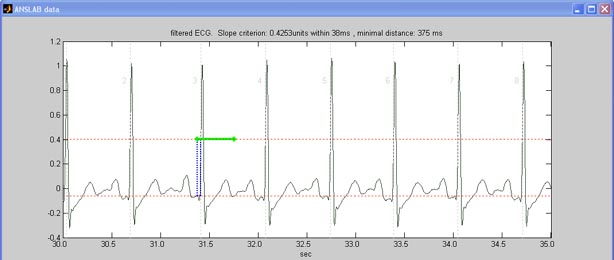
This threshold can be changed in the menu to make it more conservative (reducing false positives in noisy files) or more progressive (reducing false negatives in noisy files). You can change the amplitude difference amount (rise) and the time window in which this difference has to be reached (default: 37 ms). For very noisy data, you can try using a differentiating algorithm for r-wave detection. This method is less prone to movement artifacts and baseline drifts, and you can adjust parameters of this detection process using the given adjustment dialogs.

You can also rerun the R-wave-identification algorithm at a later point, by using the 'resume at'-dropdownmenu next to the 'resume'-button: Selecting '0' will restart at the analysis start without reloading the data. Thus, if you thoroughly edited the raw ecg signal, you can have anslab check this modified signal for R-Waves. Note that this can only be done, before analyzing T-Wave-Amplitude, because at any later stage, R-Waves will be looked for in a signal, the R-Waves of which have been removed by interpolation (see below).

Moreover, this graph can help identify sampling rate related problems: if in the displayed 5 seconds, you find more than 10 or less than 3 R-waves, odds are anslab has wrong information about the sampling rate.

After accepting (or changing) the threshold, anslab calculates the IBI time series for the entire data file. The filtered ECG and R-wave detection accuracy can be inspected by switching the display mode from 'Event' to 'Raw'. In this mode, anslab identifies the R-wave of each heartbeat with a vertical red line. The distance between vertical lines, in milliseconds, is the IBI (inter beat interval). Typical values range from about 500-1300 ms. Variations of about 200-300 ms as part of normal heart rate variability within a 5-min or so file are almost always normal. The goal of editing ECG files is to make sure that anslab has correctly identified the timing of all R-waves. For spectral analysis of heart rate variability, single spikes can seriously distort the spectral estimates. Thus, for this also certain subclinical or clinical arrhythmias (e.g., ectopic beats) need to be interpolated in some way (see below for details on r-wave-editing).

When you're happy with the r-wave-markers, hit 'resume' to continue ecg-processing. The next type of display, T-wave amplitudes, rarely requires editing since most outliers will be averaged out. After hitting 'resume' once more, you can choose 'Save reduced data' to save extracted variables to file, or 'quit' to exit editing without saving.

RSA (Respiratory Sinus Arrhythmia)
RSA generally should be analyzed in anslab using the spectral-analysis tool. You can however get a glimpse of RSA during the ecg-analysis: when the ibi has been calculated, activate the psd- option in the display-section of anslab command window. This will cause anslab to transform the IBI trace to a uniform sampling rate and run a specific kind of spectral analysis (power-spectral-density) with this new signal. RSA can then be quantified by measuring the power of  three standard frequency bands (very low frequencies: 0.025 to 0.07 Hz; low frequencies: 0.07 to 0.15 Hz; high frequencies: 0.15 to 0.5 Hz ). These bands can be visualized by activating the  rsa bands - option of the display-section. Moreover, they are displayed in the matlab command window, from where you can copy and paste the values to a text file. The PSD-analysis is run over displayed data window, allowing you to select the data segment of interest by modifying position and size of the displayed segment. Moreover, you can remove a general trend in the ibi-signal prior to psd-calculation by using the trend- and detrend-checkboxes in the display section. You can display ibi and psd simultaneously by using the  mirror active signal-menuitem in the file-menu. The graph below shows such a mirrored setup of detrended ibi-trace with rsa bands highlighted in color.

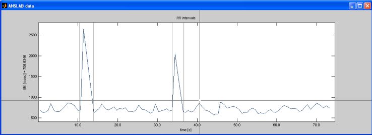
When editing, you are looking for abnormalities in height of the spikes displayed in the IBI window.  Artifacts in this data series, which appear as unusually low or high spikes, are misidentified or unidentified R-waves.  A misidentified R-wave will appear in the first window as either 2 very short IBIs or 1 very short IBI coupled with an unusually long IBI.  
If an R-wave is missing, you will see an unusually high IBI value, i.e. a high spike in the IBI series.  The IBI then typically is twice as long as average for a subject. For example, an IBI that hits a threshold greather than 1400 would suggest a missed R-wave for most subjects. anslab displays an entire file in one window. Depending on file length, artifacts may be quite obvious or more ambiguous. The shorter the file, the more subtle artifacts may appear. Always use the vertical axis (IBI in ms) when considering whether a spike in the graph is unusual. 

When you spot what appears to be an outlier in the graph, select the 'define segments' button on the command window. Then mark several suspicious areas by clicking to the left and right of the unusual signal. Blue lines will appear at these points. 

Mark all suspicious spikes this way. The best length for an interval is about 15-20 seconds. This will allow you to see both the overall pattern of R-waves and the individual irregularities. By clicking outside the axis area, you finish defining segments. Intervals will be highlighted with a grey background color.  You can then navigate between these intervals, by using the 'segment' section on the command window.  Push the '<<'-button to go to the first interval. The zoom will be set automatically so that the selected interval will fill the entire data window. Then push the 'Event/Raw'-toggle-button to switch the display so that you can see the raw ECG and actual detected R-waves as blue lines. If the interval you marked is not ideal, you can redefine intervals by selecting the 'define segments' button. If you wish to zoom out to display the total length of the loaded data before redefining segments, select the 'total interval'-button in the 'zoom'-section.

Usually, what you will find is that one of the R-waves has not been detected because of some distortion in the data. A misidentified R-wave appears as a vertical line that ‘misses’ the nearest R-wave or a vertical line, which has mistaken a movement/technical artifact for an R-wave. It is almost always obvious where an R-wave should be. Remove incorrect identifications by using the 'delete'-button in the editing section of the command window and click close to the vertical line. Insert the correct or missing R-wave with the 'insert'-button and then click in the signal where you want to insert the event. A blue line will appear, telling you that the program treats it as an R-wave now.

There are various other editing options, for a number of special problems of ecg-editing:
Insert on peak: This button looks for a local maximum near your mouse click and sets the r-wave on this maximum.
Insert interp1: If you wish to insert an r-wave marker exactly between two adjacent markers, select this button and click on the left half of the interval enclosed by the two markerks.
Insert interp2: This works exactly like 'insert interp1' except that two markers will be inserted so that the interval is evenly divided in thirds.
Insert >>>  and  <<< insert:  These two buttons are used for inserting r-wave-markers at a distance from a given marker that is decuded from preceding/subsequent present markers. If you have for instance a long interval of non-recognized r-waves, you can use these button repeatedly to fill the interval with a heart rate given before or after the blank period.
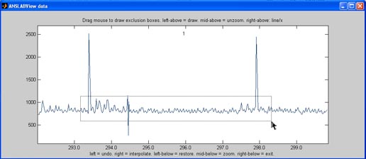
Delete box: use this option to delete multiple r-wave-markers at a time, by drawing a rectangle around them
Exclusion box: do not use this button when displaying ecg raw data, as it serves to modify the signal itself, not the r-wave-markes.
Inclusion box: this option is meant to help you include multiple non-recognized r-waves, that in general have a normal waveform, but were missed by the identifaction algorithm. Draw a rectangle around the maxima of these r-waves, ignoring already recognized r-waves. anslab will insert one event marker for each lokal maximum found inside your selection box, that has a minimum distance to present markers.

By hitting ">" in the segment-section, you can directly go to the next area you previously marked as suspicious (if any). Here you repeat what you’ve done above. The distance between R-waves does not have to be uniform, as long as the cycle is correct. Usually it is not recommended to remove R-waves that have been correctly identified to make the distance between them even, unless they are due to arrhythmic cardiac activity and you later want to analyze heart rate variability.  
If you switch back to the 'Event'-display, anslab will redisplay the IBI window with the changes you have made. If you have edited correctly, the unusual spikes and dips should no longer appear. If there are new abnormal spikes, you can go through the editing process again; sometimes, smaller artifacts that were not as prominent in the first window now show up as unusual. 

A quick kind of outlier editing is the 'connect'-button, which for the ibi-trace works differently than for other signal types (and only at the first analysis resume point). Use it to draw a rectangle around the good part of the data. Values outside the drawn rectangle will be interpolated. Moreover, and this is the special part of the connect-tool with the ibi-trace, R-Wave markers are inserted on the raw channel at corresponding locations.  

When you are satisfied that you have made all necessary corrections, hit 'resume' in the 'settings'-section of the command window to carry on.

Next, the TWA (T-wave amplitude) will be displayed:

Suspicious areas can be looked at similarly to IBI editing by using the 'redefine segments'-button.

The T-waves are marked in red, the place where the R-wave was detected (but is now cut out) is marked in grey in the lower graph, that shows the original ECG. Here, you should focus on misdetected T-waves, mostly due to artifacts. Those will often be manifested by outliers, i.e. spikes. Go to the suspicious intervals. If in the data you cannot detect the T-wave (zoom in to make sure), but the program has detected T-waves, you should delete those. To do that, you can either use the 'delete'-button as for R-wave-editing, or you can use the 'exlusion box'-button.  You do not have to be very accurate because typically the averaging over periods will overcome single outliers. Generally, you don’t have to insert any events. If you are done, push 'resume'  and select "Save reduced data (existing files will be overwritten)" if you want to save your changes. That's it!

The most important element of ECG editing is consistent and accurate identification of R-waves. Unlike other parameters that are often just used to compute means over minutes or so, any outlier in the IBI affects the quality of the heart rate variability analysis.

What Do I Do When anslab Does Not Identify Any R-waves?  Sometimes the ECG is unusual so that the standard detection parameters do not work well. In anslab, you will see a window that shows extremely long intervals between R-waves. Or, anslab will display a straight line if no R-waves have been detected. This is a frustrating problem but easy to solve. Instead of manually inserting every R-wave, you can choose another threshold for R-spike detection. Or (for more advanced Matlab users), you can select in the header of the the R-spike detection program to use other settings for the detection algorithm.

For example: High pass filtering on/off, Cutoff frequency in Hz (e.g., 2), Reversal of signal (e.g., yes, if the R-spike is downward), Detection window size (e.g., 150 sample points). If change in these settings do not significantly increase the number of R-waves identified, you can experiment raising or lowering ‘Backward Comparison Point’ and ‘Increase from point in mV’. Backward comparison point (e.g., 8 sample points).Increase from point in mV (e.g., 0.005).

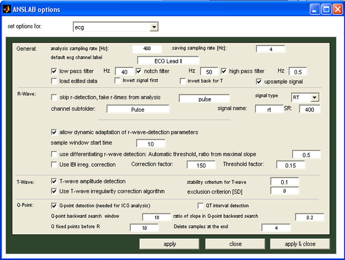
Extended options

If you want to open already edited data, please check the "load edited data" box (anslab will look for the file ...\EXP\ecg\ECG Lead II\EXP130300.mat).

For cases, where no ecg-measurement is available, and the heart rate is calculated from a different cardiovascular channel such a pulse or blood pressure, you can still  use the ecg-module for ibi-editing purposes. To do this, check the 'skip r-wave detection, take r-times from analysis'-option  on the ecg-tab of anslab options dialog, and enter the alternative analysis name, the channel subfolder name, the signal name, the signal type and the sampling rate of the signal to allow anslab to load the r-wave times from a different file. The options shown are an example of how r-wave times can be loaded from a previously performed non-ecg-based pulse analysis: when opening a raw data file ( e.g. the file EXP01303.txt of an experiment EXP) for ecg-analysis, anslab will not try to load ecg-raw-data from the data file, but look for a mat-file in the directory    ...\pulse\Pulse\  inside your study folder,  that belongs to the same subject (13) and run (3)  and has been processed as one entire datafile (adding 00 as segment number to the file name, thus anslab will look for the file ...\EXP\pulse\Pulse\EXP0130300.mat )  and try to load the variable 'rt' from this file, assuming the r-time-values are given as points sampled at 400 Hz. You can then edit r-time-signal and save it by hitting the resume-button. As no raw-data is loaded, however, no data is displayed when switching to 'RAW'-mode, except the r-wave-markers when zooming in sufficiently.